Asteroid Tracking Simulation

In tracking mode, the telescope slews to follow a moving target — the asteroid stays fixed as a point source while background stars trail across the detector.

This notebook simulates that scenario across 5 consecutive exposures of the near-Earth asteroid 2024 MK, using real ephemerides from JPL Horizons.

1. Fetch the ephemeris from JPL Horizons

We query Horizons for the asteroid’s sky position and angular velocity at the mid-time of each exposure. The cadence is exposure_time + processing_time seconds.

from astropy.time import Time, TimeDelta
from astroquery.jplhorizons import Horizons

start_time = Time("2024-06-29T13:00:00", format="isot")
exposure_time = 5.0  # seconds
processing_time = 1.0  # seconds
n_exposures = 5

epochs = [
    (start_time + TimeDelta(i * (exposure_time + processing_time), format="sec")).jd
    for i in range(n_exposures)
]

# A bright near-Earth asteroid with significant motion during the exposures
target_id = "2024 MK"
location = "807"  # Cerro Paranal (ESO)

obj = Horizons(id=target_id, location=location, epochs=epochs)
eph = obj.ephemerides()

The columns we need are RA, DEC, the angular velocity components, and the visual magnitude. Horizons returns RA_rate as the on-sky rate dα·cos(δ)/dt in arcsec/hour — that is, the actual angular speed projected along the RA direction, not the raw coordinate rate.

from astropy import units as u

eph["datetime_str", "RA", "DEC", "RA_rate", "DEC_rate", "V"].pprint()

ra = eph["RA"].value * u.deg
dec = eph["DEC"].value * u.deg
ra_rate = eph["RA_rate"].value * u.arcsec / u.hour  # on-sky: dα·cos(δ)/dt
dec_rate = eph["DEC_rate"].value * u.arcsec / u.hour
visual_magnitude = eph["V"].value

      datetime_str           RA       DEC     RA_rate    DEC_rate    V  
          ---               deg       deg    arcsec / h arcsec / h  mag 
------------------------ --------- --------- ---------- ---------- -----
2024-Jun-29 13:00:00.000 291.85454 -14.97028   16665.78   16834.32 9.384
2024-Jun-29 13:00:06.000 291.86255  -14.9625   16665.93   16835.22 9.384
2024-Jun-29 13:00:12.000 291.87055 -14.95473   16666.08   16836.13 9.385
2024-Jun-29 13:00:18.000 291.87856 -14.94695   16666.23   16837.03 9.385
2024-Jun-29 13:00:24.000 291.88656 -14.93917   16666.37   16837.93 9.385

2. Create the moving source

We wrap the asteroid into a Sources object. The flux is converted from visual magnitude using an arbitrary zero-point of 22.5.

Sources.ra_rates follows the same on-sky dα·cos(δ)/dt convention as Horizons, so we can pass the rates directly — attaching astropy units lets cabaret convert from arcsec/hour to the internal arcsec/s automatically.

import cabaret

asteroid = cabaret.Sources.from_arrays(
    ra=ra,
    dec=dec,
    fluxes=10 ** (-0.4 * (visual_magnitude - 22.5)),
    ra_rates=ra_rate,
    dec_rates=dec_rate,
)

3. Generate the simulated images

For each exposure we:

1. Point the telescope at the asteroid’s current position (ra[i], dec[i]).

2. Set tracking_ra_rate / tracking_dec_rate so the telescope follows the asteroid — stars therefore drift across the detector during the exposure.

3. Inject the asteroid as an additional_sources on top of the Gaia star field.

The tracking rates use the same on-sky arcsec/s convention.

observatory = cabaret.Observatory()

images = [
    observatory.generate_image(
        ra=ra[i],
        dec=dec[i],
        tracking_ra_rate=ra_rate[i],  # on-sky: dα·cos(δ)/dt
        tracking_dec_rate=dec_rate[i],
        exp_time=exposure_time,
        additional_sources=asteroid[i : i + 1],
    )
    for i in range(n_exposures)
]

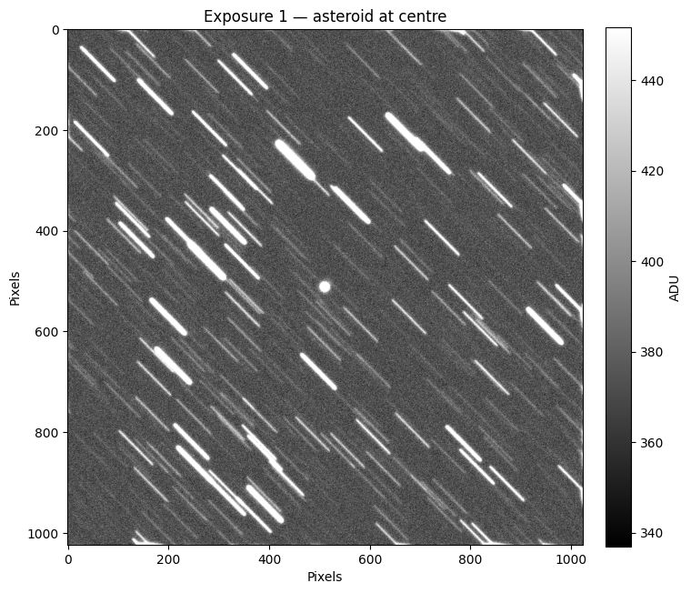
4. Inspect a single frame

The asteroid should appear as a sharp point source at the image centre, while background stars are smeared into short trails in the direction opposite to the asteroid’s motion.

from cabaret.plot import plot_image

_ = plot_image(images[0], title="Exposure 1 — asteroid at centre")

5. Animate all exposures

All frames share the same colour scale (1st–99.9th percentile across the whole stack) so brightness is directly comparable between exposures.

import matplotlib.pyplot as plt
import numpy as np
from IPython.display import HTML
from matplotlib.animation import ArtistAnimation

vmin, vmax = np.percentile(np.stack(images), [1, 99.9])

fig, ax = plt.subplots(figsize=(7, 6))
fig.subplots_adjust(right=0.82)
plot_image(images[0], ax=ax, vmin=vmin, vmax=vmax)

frames = []
for i, img in enumerate(images):
    im = ax.imshow(img, cmap="gray", vmin=vmin, vmax=vmax, animated=True)
    label = ax.text(
        0.5,
        1.02,
        f"Exposure {i + 1} of {n_exposures}",
        transform=ax.transAxes,
        ha="center",
        fontsize=12,
        fontweight="bold",
    )
    frames.append([im, label])


ani = ArtistAnimation(fig, frames, interval=600, blit=True)
plt.close()
HTML(ani.to_jshtml())

Once Loop Reflect